Understanding the Vanishing Gradient Problem and the Role of Activation Functions

Deep learning has revolutionized many fields, from computer vision to natural language processing. However, training deep neural networks presents unique challenges, one of which is the vanishing gradient problem. This issue can impede the learning process, making it difficult to train deep models effectively. In this article, we’ll explore what the vanishing gradient problem is, how it arises, and the crucial role activation functions play in addressing it.

What is the Vanishing Gradient Problem?

The vanishing gradient problem occurs during the training of deep neural networks, particularly those with many layers. To understand it, let’s first revisit how neural networks learn.

Backpropagation and Gradients

Neural networks learn through a process called backpropagation, where the model adjusts its weights based on the error of its predictions. This adjustment is guided by the gradients of the loss function with respect to the model’s parameters. These gradients are calculated using the chain rule of calculus, propagating from the output layer back to the input layer.

In a deep network, this backpropagation process involves the multiplication of many derivatives (gradients) corresponding to each layer’s weights. If these gradients are small, they can shrink exponentially as they move backward through the network. This results in gradients that are near zero by the time they reach the initial layers, effectively “vanishing” and preventing these layers from learning.

Why is the Vanishing Gradient Problem a Big Deal?

When gradients vanish, the initial layers of the network learn very slowly or not at all. This is problematic because these layers are typically responsible for detecting low-level features in data, which are crucial for building more complex representations in subsequent layers. If the early layers don’t learn effectively, the entire network’s performance suffers.

The Role of Activation Functions

Activation functions introduce non-linearity into the network, enabling it to learn complex patterns. However, the choice of activation function can significantly impact the severity of the vanishing gradient problem.

Sigmoid and Tanh: The Culprits

The sigmoid and tanh activation functions were commonly used in early neural networks. Unfortunately, these functions are particularly prone to causing vanishing gradients.

Sigmoid: The sigmoid function squashes input values into a range between 0 and 1, defined as:

sigmoid function

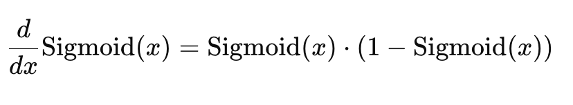
derivative of the sigmoid functionThe derivative ranges from 0 to 0.25, with the maximum value at x=0. This small range of derivatives, especially when x is very large or very small, leads to vanishing gradients.

Tanh: The tanh function is similar to sigmoid but squashes input values into a range between -1 and 1, defined as:

tanh function

derivative of tanhThe derivative ranges from 0 to 1, with the maximum value at x=0x = 0x=0. Similar to sigmoid, the derivative diminishes as xxx moves away from zero, leading to vanishing gradients.

ReLU: A Breakthrough

The introduction of the Rectified Linear Unit (ReLU) activation function marked a significant advancement in mitigating the vanishing gradient problem. Unlike sigmoid and tanh, ReLU is defined as:

ReLU function

derivative of the ReLU functionThe derivative is either 0 or 1, meaning the gradient does not diminish as quickly during backpropagation, allowing deeper networks to learn more effectively. However, the zero derivative for negative inputs can lead to the “dying ReLU” problem.

Variants of ReLU

ReLU has its own limitations, such as the “dying ReLU” problem, where neurons can become inactive if they consistently output zero. This issue has led to the development of several ReLU variants:

Leaky ReLU: Allows a small, non-zero gradient for negative inputs, defined as:

Leaky ReLU function

derivative of Leaky ReLU functionThe derivative is either 1 or a small positive value α\alphaα (typically 0.01), which helps prevent neurons from dying.

Parametric ReLU (PReLU): Introduces learnable parameters to control the slope of the negative part of the function:

Parametric ReLU function

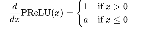
derivative of Parametric ReLU functionThe range depends on the learned parameter aaa, typically greater than 0.

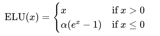
Exponential Linear Unit (ELU): Smooths the transition to negative values, defined as:

ELU function

derivative of ELU functionThe derivative is 1 for positive inputs and a small positive value for negative inputs, helping the network learn more effectively.

Beyond ReLU: Advanced Activation Functions

In addition to ReLU and its variants, other advanced activation functions have been proposed to address the vanishing gradient problem further:

Swish: A smooth function defined as:

swish function

derivative of the Swish functionThe range is more flexible than ReLU, providing non-zero derivatives for a wider range of inputs, which can benefit some networks.

GELU (Gaussian Error Linear Unit): Combines properties of both linear and non-linear activations, defined as:

GELU functionwhere Φ(x) is the cumulative distribution function of the Gaussian distribution.

derivative of the GELU functionwhere ϕ(x) is the probability density function of the Gaussian distribution.

The derivative is smooth and non-zero across a wide range of inputs, which can lead to better performance in deep networks.

*This post originally appeared on my Medium

.*